Implementation Details: TRANSIC's Simulation Training and Real-World Data Collection

Table of Links

Abstract and 1 Introduction

2 Preliminaries

3 TRANSIC: Sim-to-Real Policy Transfer by Learning from Online Correction and 3.1 Learning Base Policies in Simulation with RL

3.2 Learning Residual Policies from Online Correction

3.3 An Integrated Deployment Framework and 3.4 Implementation Details

4 Experiments

4.1 Experiment Settings

4.2 Quantitative Comparison on Four Assembly Tasks

4.3 Effectiveness in Addressing Different Sim-to-Real Gaps (Q4)

4.4 Scalability with Human Effort (Q5) and 4.5 Intriguing Properties and Emergent Behaviors (Q6)

5 Related Work

6 Conclusion and Limitations, Acknowledgments, and References

A. Simulation Training Details

B. Real-World Learning Details

C. Experiment Settings and Evaluation Details

D. Additional Experiment Results

A Simulation Training Details

In this section, we provide details about simulation training, including the used simulator backend, task designs, reinforcement learning (RL) training of teacher policy, and student policy distillation.

A.1 The Simulator

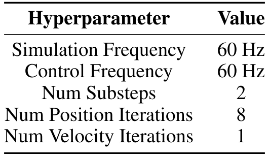
We use Isaac Gym Preview 4 [10] as the simulator backend. NVIDIA PhysX[1] is used as the physics engine to provide realistic and precise simulation. Simulation settings are listed in Table A.I. The robot model is from Franka ROS package[2]. We borrow furniture models from FurnitureBench [90] to create various tasks that require complex and contact-rich manipulation.

A.2 Task Implementations

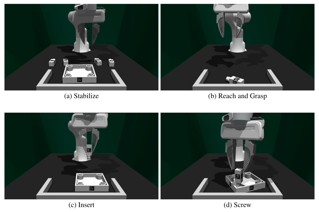
We implement four tasks based on the furniture model square table: Stabilize, Reach and Grasp, Insert, and Screw. An overview of simulated tasks is shown in Fig A.1. We elaborate on their initial conditions, success criteria, reward functions, and other necessary information.

A.2.1 Stabilize

In this task, the robot needs to push the square tabletop to the right corner of the wall such that it is supported and remains stable in following assembly steps. The robot is initialized such that its gripper locates at a neutral position. The tabletop is initialized at the coordinate (0.54, 0.00) relative to the robot base. We then randomly translate it with displacements drawn from U(−0.015, 0.015) along x and y directions (the distance unit is meter hereafter). We also apply random Z rotation with values drawn from U(−15°, 15°). Four table legs are initialized in the scene. The task is successful only when the following three conditions are met:

1. The square tabletop contacts the front and right walls;

2. The square tabletop is within a pre-defined region;

3. No table leg is in the pre-defined region.

A.2.2 Reach and Grasp

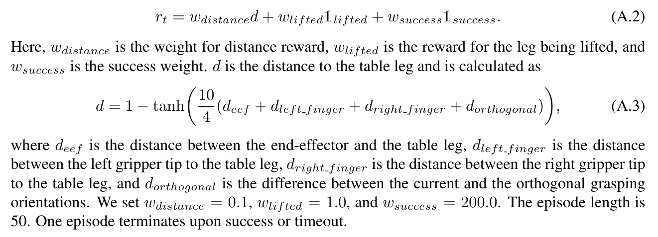
In this task, the robot needs to reach and grasp a table leg that is randomly spawned in the valid workspace region. The task is successful once the robot grasps the table leg and lifts it for a certain

height. The object’s irregular shape limits certain grasping poses. For example, the end-effector needs to be near orthogonal to the table leg in the xy plane and far away from the screw thread. Therefore, we design a curriculum over the object geometry to warm up the RL learning. It gradually adjusts the object geometry from a cube, to a cuboid, and finally the table leg. In all curriculum stages, the reward function is

A.2.3 Insert

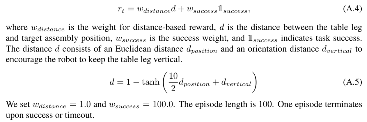
In this task, the robot needs to insert a pre-grasped table leg into the far right assembly hole of the tabletop, while the tabletop is already stabilized. The tabletop is initialized at the coordinate (0.53, 0.05) relative to the robot base. We then randomly translate it with displacements sampled from U(−0.02, 0.02) along x and y directions. We also apply random Z rotation with values drawn from U(−45°, 45°). We further randomize the robot’s pose by adding noises sampled from U(−0.25, 0.25) to joint positions. The task is successful when the table leg remains vertical and is close to the correct assembly position within a small threshold. We design curricula over the randomization strength to facilitate the learning. The following reward function is used:

A.2.4 Screw

In this task, the robot is initialized such that its end-effector is close to an inserted table leg. It needs to screw the table leg clockwise into the tabletop. We design curricula over the action space: at the early stage, the robot only controls the end-effector’s orientation; at the latter stage, it gradually takes full control. We slightly randomize object and robot poses during initialization. The reward function is

A.3 Teacher Policy Training

A.3.1 Model Details

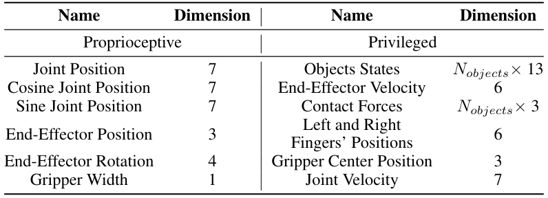
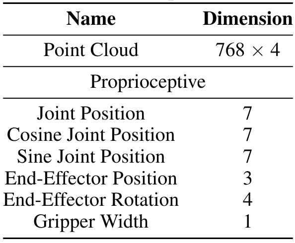
Observation Space Besides proprioceptive observations, teacher policies also receive privileged observations to facilitate the learning. They include objects’ states (poses and velocities), endeffector’s velocity, contact forces, gripper left and right fingers’ positions, gripper center position, and joint velocities. Full observations are summarized in Table A.II.

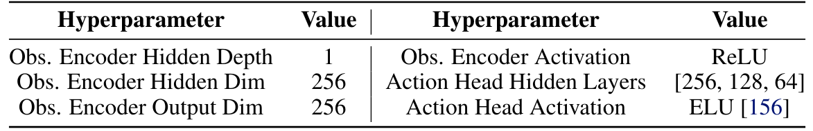
Model Architecture We use feed-forward policies [155] in RL training. It consists of MLP encoders to encode proprioceptive and privileged vector observations, and unimodal Gaussian distributions as the action head. Model hyperparameters are listed in Table A.III.

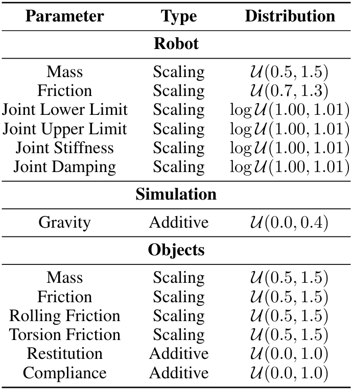
A.3.2 Domain Randomization

We apply domain randomization during RL training to learn more robust teacher policies. Parameters are summarized in Table A.IV.

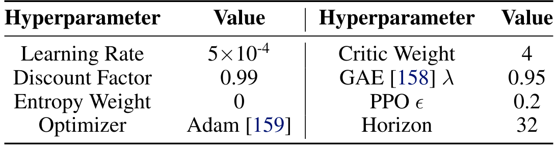
A.3.3 RL Training Details

We use the model-free RL algorithm Proximal Policy Optimization (PPO) [84] to learn teacher policies. Hyperparameters are listed in Table A.V. We customize the framework from Makoviichuk and Makoviychuk [157] to use as our training framework.

A.4 Student Policy Distillation

A.4.1 Data Generation

We use trained teacher policies as oracles to generate data for student policies training. Concretely, we roll out each teacher policy to generate 10, 000 successful trajectories for each task. We exclude trajectories that are shorter than 20 steps.

A.4.2 Observation Space

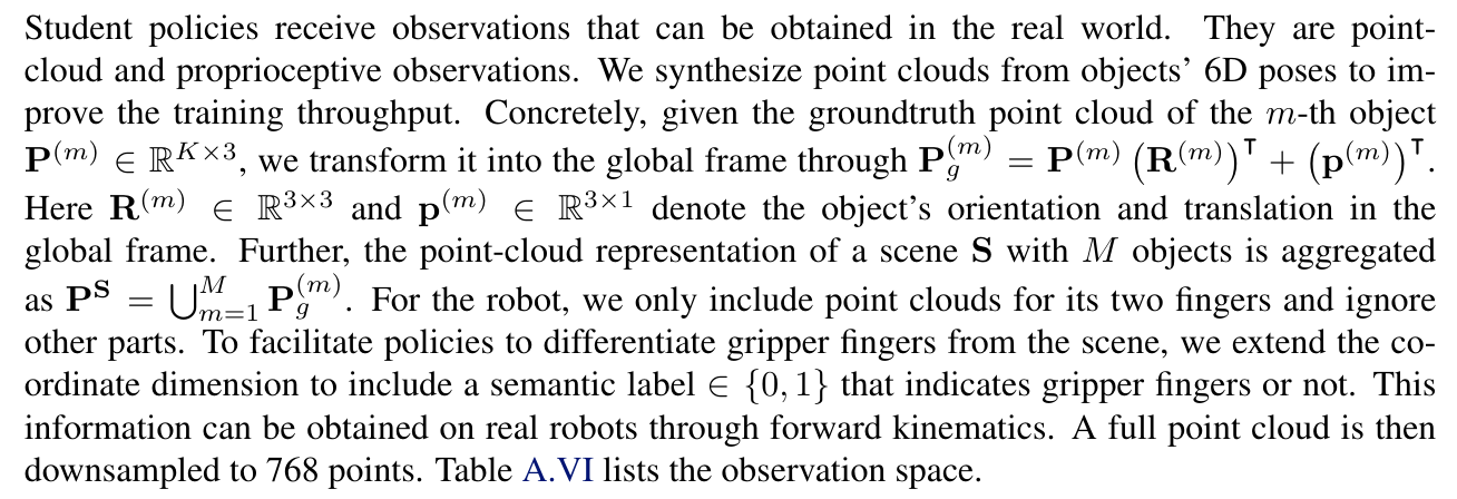
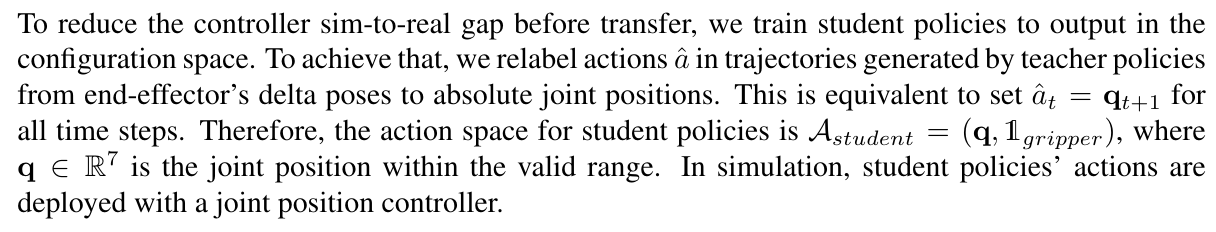
A.4.3 Action Space Distillation

A.4.4 Model Architecture

We use feed-forward policies for tasks Reach and Grasp and Insert and recurrent policies for tasks Stabilize and Screw as we find they achieve the best distillation results. PointNets [86] are used to encode point clouds. Recall that each point in the point cloud also contains a semantic label indicating the gripper or not. We concatenate point coordinates with these semantic labels’ vector embeddings before passing into the PointNet encoder. We use Gaussian Mixture Models (GMM) [68] as the action head. Detailed model hyperparameters are listed in Table A.VII.

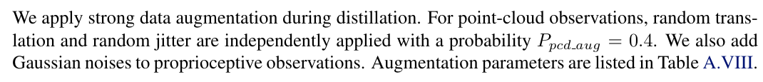
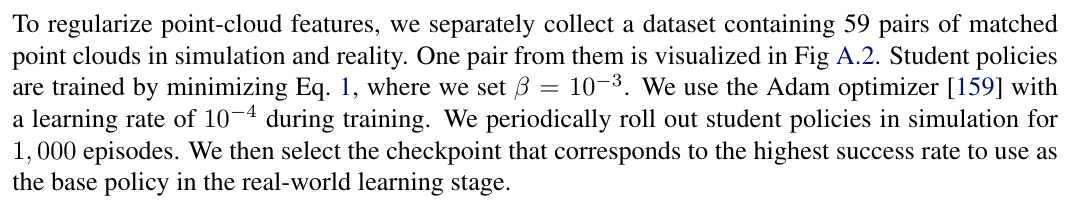
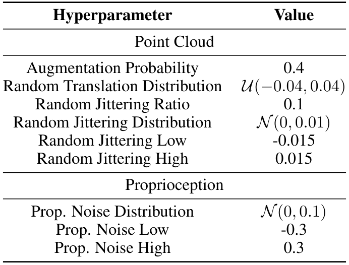
A.4.5 Data Augmentation

A.4.6 Training Details

B Real-World Learning Details

In this section, we provide details about real-world learning, including the hardware setup, humanin-the-loop data collection, and residual policy training.

B.1 Hardware Setup

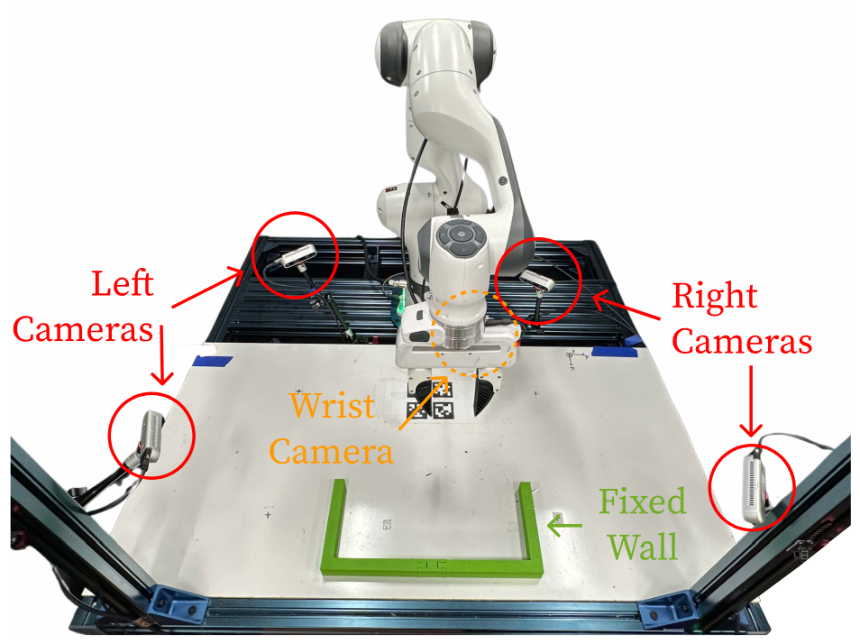
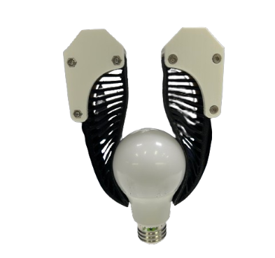
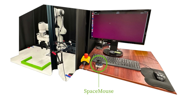
As shown in Fig. A.3, our system consists of a Franka Emika 3 robot mounted on the tabletop. We use four fixed cameras and one wrist camera for point cloud reconstruction. They are three RealSense D435 and two RealSense D415. There is also a 3d-printed three-sided wall glued on top of the table to provide external support. We use a soft gripper for better grasping (Fig A.4). We use a joint position controller from the Deoxys library [162] to control our robot at 1000 Hz.

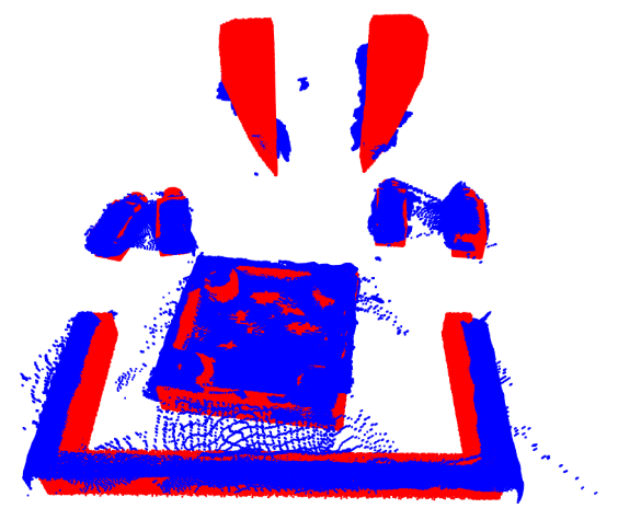
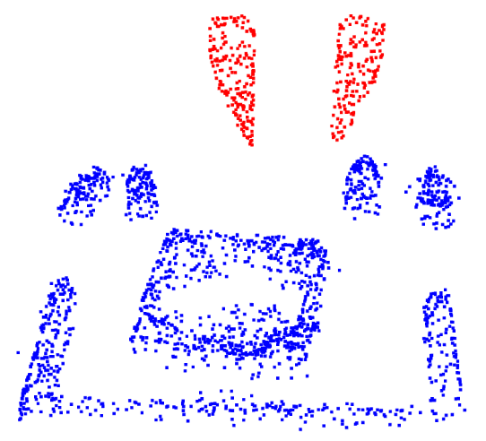
B.2 Obtaining Point Clouds from Multi-View Cameras

We use multi-view cameras for point cloud reconstruction to avoid occlusions. Specifically, we first calibrate all cameras to obtain their poses in the robot base frame. We then transform captured point clouds in camera frames to the robot base frame and concatenate them together. We further perform cropping based on coordinates and remove statistical and radius outliers. To identify points belonging to the gripper so that we can add gripper semantic labels (Sec. A.4.2), we compute poses for two gripper fingers through forward kinematics. We then remove measured points corresponding to gripper fingers through K-nearest neighbor, given fingers’ poses and synthetic point clouds. Subsequently, we add semantic labels to points belonging to the scene and synthetic gripper’s point clouds. Finally, we uniformly down-sample without replacement. We opt to not use farthest point sampling [163] due to its slow speed. One example is shown in Fig. A.5.

B.3 Human-in-the-Loop Data Collection

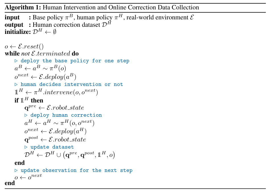
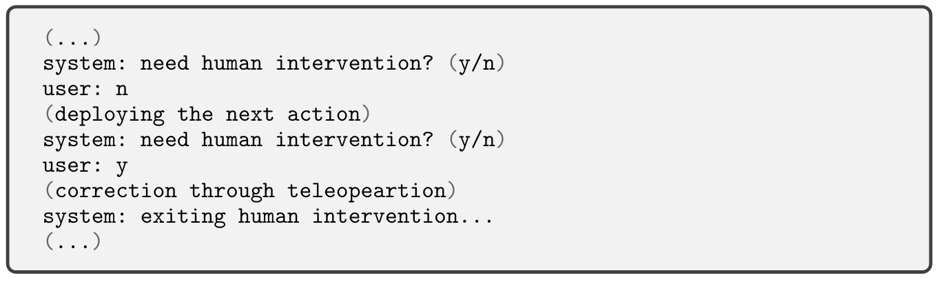
This data collection procedure is illustrated in Algorithm 1. As shown in Fig. A.6, we use a 3Dconnexion SpaceMouse as the teleoperation device. We design a specific UI (Fig. A.7) to facilitate the synchronized data collection. Here, the human operator will be asked to intervene or not. The operator answers through keyboard. If the operator does not intervene, the base policy’s next action will be deployed. If the operator decides to intervene, the SpaceMouse is then activated to teleoperate the robot. After the correction, the operator can exit the intervention mode by pressing one button on the SpaceMouse. We use this system and interface to collect 20, 100, 90, and 17 trajectories with correction for tasks Stabilize, Reach and Grasp, Insert, and Screw, respectively. We use 90% of them as training data and the remaining as held-out validation sets. We visualize the cumulative distribution function of human correction in Figure A.8.

B.4 Residual Policy Training

B.4.1 Model Architecture

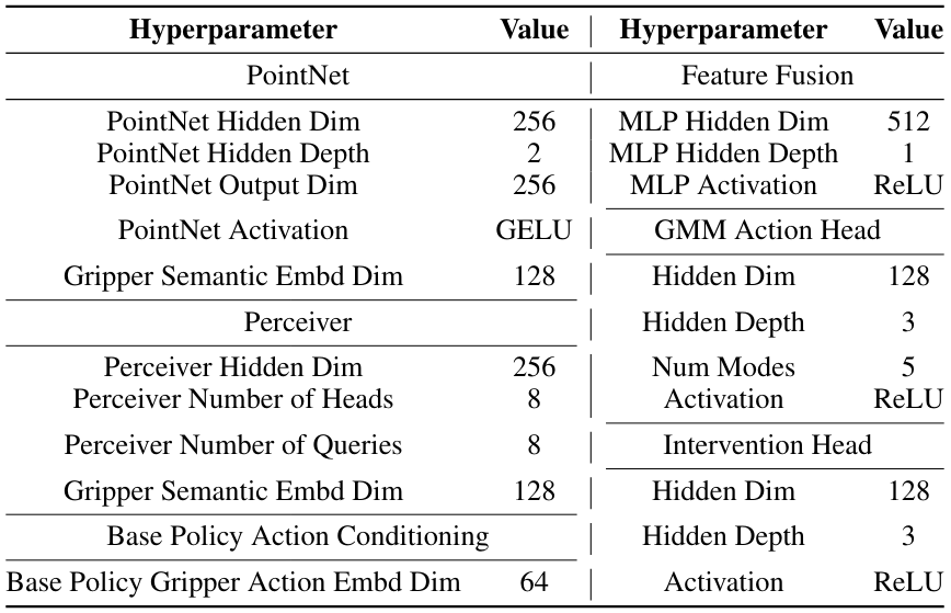
The residual policy takes the same observations as the base policy (Table A.VI). Furthermore, to effectively predict residual actions, it is also conditioned on base policy’s outputs. Its action head outputs eight-dim vectors, while the first seven dimensions correspond to residual joint positions and the last dimension determines whether to negate base policy’s gripper action or not. Besides, a separate intervention head predicts whether the residual action should be applied or not (learned gated residual policy, Sec. 3.3).

For tasks Stabilize and Insert, we use a PointNet [86] as the point-cloud encoder. For tasks Reach and Grasp and Screw, we use a Perceiver [87, 88] as the point-cloud encoder. Residual policies are instantiated as feed-forward policies in all tasks. We use GMM as the action head and a simple two-way classifier as the intervention head. Model hyperparameters are summarized in Table A.IX

B.4.2 Training Details

To train the learned gated residual policy, we first only learn the feature encoder and the action head. We then freeze the entire model and only learn the intervention head. We opt for this two-stage training since we find that training both action and intervention heads at the same time will result in sub-optimal residual action prediction. We follow the best practice for policy training [98, 155, 164], including using learning rate warm-up and cosine annealing [89]. Training hyperparameters are listed in Table A.X.

[1] https://developer.nvidia.com/physx-sdk

[2] https://github.com/frankaemika/franka_ros